14 Intermediate SQL

join Expressions
view definition
integrity constraints
more details regarding data definition
authorization

14.1 Join Expressions

14.1.1 Natural join

corresponds to $\bowtie$. Consider:

select *
from (
    values 
    (1, 2),
    (3, 2)
) r(a, b) natural join
(
    values 
    (2, 3),
    (2, 4),
    (1, 10),
    (5, 8)
) s(b, c)

4 records
b	a	c
2	3	3
2	1	3
2	3	4
2	1	4

14.1.2 Join Using

Possible to explicitely list attributes on which it is to be joined:

select *
from (
    values 
    (1, 2, 5),
    (3, 2, 7)
) r(a, b, c) join
(
    values 
    (2, 3),
    (2, 4),
    (1, 10),
    (5, 8)
) s(b, c) using (b)

4 records
b	a	c	c..4
2	3	7	3
2	1	5	3
2	3	7	4
2	1	5	4

same as

select *
from r, s
where r.b = s.b

14.1.3 Join on

select *
from student join takes on student.id = takes.student_id

Displaying records 1 - 10
id	name	dept_name	tot_cred	student_id	course_id	sec_id	semester	year	grade
00128	Zhang	Comp. Sci.	102	00128	CS-101	1	Fall	2017	A
00128	Zhang	Comp. Sci.	102	00128	CS-347	1	Fall	2017	A-
12345	Shankar	Comp. Sci.	32	12345	CS-101	1	Fall	2017	C
12345	Shankar	Comp. Sci.	32	12345	CS-190	2	Spring	2017	A
12345	Shankar	Comp. Sci.	32	12345	CS-315	1	Spring	2018	A
12345	Shankar	Comp. Sci.	32	12345	CS-347	1	Fall	2017	A
19991	Brandt	History	80	19991	HIS-351	1	Spring	2018	B
23121	Chavez	Finance	110	23121	FIN-201	1	Spring	2018	C+
44553	Peltier	Physics	56	44553	PHY-101	1	Fall	2017	B-
45678	Levy	Physics	46	45678	CS-101	1	Fall	2017	F

Exactly the same as

select *
from student, takes
where student.id = takes.student_id

Advantages:

readability in separating join conditions from other where-clause conditions
necessary for outer joins.

14.1.4 Outer Joins

According to the definition of usual join operation

select *
from student join takes
on student.id = takes.student_id

non-matched tuples don’t appear in the resulting relation. But sometimes we might nevertheless wich to include such tuples in the result.

This can be achieved by

left outer join
right outer join
full outer join

First of all, notice that there is one student who hasn’t taken any courses:

select *
from student s 
where s.id not in (
    select t.student_id 
    from takes t 
)

2 records
id	name	dept_name	tot_cred
70557	Snow	Physics	0
12789	Newman	Comp. Sci.	NA

An he doesn’t appear in the previous join operation. We can include this student in the final result using left outer join:

select *
from student s left outer join takes t 
on s.id = t.student_id 
order by s.id desc

Displaying records 1 - 10
id	name	dept_name	tot_cred	student_id	course_id	sec_id	semester	year	grade
98988	Tanaka	Biology	120	98988	BIO-301	1	Summer	2018	NA
98988	Tanaka	Biology	120	98988	BIO-101	1	Summer	2017	A
98765	Bourikas	Elec. Eng.	98	98765	CS-101	1	Fall	2017	C-
98765	Bourikas	Elec. Eng.	98	98765	CS-315	1	Spring	2018	B
76653	Aoi	Elec. Eng.	60	76653	EE-181	1	Spring	2017	C
76543	Brown	Comp. Sci.	58	76543	CS-319	2	Spring	2018	A
76543	Brown	Comp. Sci.	58	76543	CS-101	1	Fall	2017	A
70557	Snow	Physics	0	NA	NA	NA	NA	NA	NA
55739	Sanchez	Music	38	55739	MU-199	1	Spring	2018	A-
54321	Williams	Comp. Sci.	54	54321	CS-101	1	Fall	2017	A-

Notice how the tuple corresponding to student Snow who hasn’t taken any courses has null values for all attributes that come from the takes relation.

Consider a simpler exampe. Consider tables:

with r(a, b) as (
    values 
    (1, 2),
    (2, 2),
    (5, 3)
), s(b, c) as (
    values
    (2, 4),
    (2, 5)
) 
select *
from r natural join s

4 records
b	a	c
2	1	5
2	1	4
2	2	5
2	2	4

Above natural join didn’t include the tuple (5, 3) from r, since it didn’t match with anything from s. But

with r(a, b) as (
    values 
    (1, 2),
    (2, 2),
    (5, 3)
), s(b, c) as (
    values
    (2, 4),
    (2, 5)
) 
select r.a a, r.b b, s.c c
from r natural left outer join s

5 records
a	b	c
1	2	5
1	2	4
2	2	5
2	2	4
5	3	NA

contains tuple (5, 3, null).

inner join is just another name for all other default joins that don’t include nonmatched tuples.

Alternative way to find students that haven’t taken a course using outer join:

select * 
from student s left outer join takes t 
on s.id = t.student_id 
where t.course_id is null

2 records
id	name	dept_name	tot_cred	student_id	course_id	sec_id	semester	year	grade
70557	Snow	Physics	0	NA	NA	NA	NA	NA	NA
12789	Newman	Comp. Sci.	NA	NA	NA	NA	NA	NA	NA

right outer join is symmetric to left outer join. Adding (4, 7) to s in the previous simple example:

with r(a, b) as (
    values 
    (1, 2),
    (2, 2),
    (5, 3)
), s(b, c) as (
    values
    (2, 4),
    (2, 5),
    (4, 7)
) 
select *
from r natural right outer join s

5 records
b	a	c
2	2	4
2	1	4
2	2	5
2	1	5
4	NA	7

(4, 7) didn’t match with any tuple from r but was still included in the result with a set null.

full outer join is a combination of left and right outer joins. Again the previous example:

with r(a, b) as (
    values 
    (1, 2),
    (2, 2),
    (5, 3)
), s(b, c) as (
    values
    (2, 4),
    (2, 5),
    (4, 7)
) 
select *
from r natural full outer join s

6 records
b	a	c
2	1	5
2	1	4
2	2	5
2	2	4
3	5	NA
4	NA	7

Anotheer full outer join exmaple:

all students from the Comp. Sci. department, along with course sections, if any that they have taken in Spring 2017; all course sections from Spring 2017 must be displayed even if no student from the Comp. Sci department has taken the course:

select s.id, t.course_id
from ( -- subquery computing relation containing students from CS department
    select s.id, s.name
    from student s 
    where s.dept_name = 'Comp. Sci.'
) s(id, name) right outer join 
( -- subquery computing relation of section taken in Spring 2017
    select t.student_id, t.course_id, t.sec_id, t.semester, t."year"
    from takes t 
    where t.semester = 'Spring'
        and t.year = 2017
) t(id, course_id, sec_id, semester, year) on s.id = t.id

3 records
id	course_id
12345	CS-190
54321	CS-190
NA	EE-181

or an equivalent alternative formulation using with to factor the subqueries:

with s(id) as (
    select s.id
    from student s 
    where s.dept_name = 'Comp. Sci.' 
), t(id, sec_id, course_id, semester, year) as (
    select t.student_id, t.sec_id, t.course_id , t.semester, t."year" 
    from takes t 
    where t.semester = 'Spring' and t."year" = 2017
)
select s.id, t.course_id 
from s right outer join t on s.id = t.id

Warning

Note that

select s.id, t.course_id
from student s right outer join takes t
on s.id = t.student_id 
where s.dept_name = 'Comp. Sci.'
    and t.semester = 'Spring'
    and t."year" = 2017

2 records
id	course_id
12345	CS-190
54321	CS-190

would be a wrong solution, since right outer join is performed before the where clause on the full student relation and not on the student relation restricted to the CS department.

To verify previous solution compute sections offered in Spring 2017:

select *
from section 
where year = 2017
    and semester = 'Spring'

3 records
course_id	id	semester	year	building	room_number	time_slot_id
CS-190	1	Spring	2017	Taylor	3128	E
CS-190	2	Spring	2017	Taylor	3128	A
EE-181	1	Spring	2017	Taylor	3128	C

Indeed, course ‘EE-181’ hasn’t been taken by any student from the CS department.

14.2 Views

Two reasons:

Security; restricting what users can see
Virtual tables that better correspond to the intuition of the user

view can be thought of extending with beyond use in a single query. It is possible to define arbitrarily many views on top of existing relations.

14.2.1 View Definition and Usage

Syntax:

create view v as <query expression>

Examples:

restricted access to instuctor relation without salary information:

create view faculty as
    select i.id, i."name" , i.dept_name 
    from instructor i

Then, we can access faculty as if it were a regular relation:

select * 
from faculty f

Displaying records 1 - 10
id	name	dept_name
10101	Srinivasan	Comp. Sci.
12121	Wu	Finance
15151	Mozart	Music
22222	Einstein	Physics
32343	El Said	History
33456	Gold	Physics
45565	Katz	Comp. Sci.
58583	Califieri	History
76543	Singh	Finance
76766	Crick	Biology

In authorization section we can see how users can be given access to views instead of or in addition to relations.

Note

view relations are not pre-computed and stored; they are computed dynamically.

view of all course section offered by the physics department in fall 2017:

create view physics_fall_2017 as 
    select c.id as course_id, s.id as section_id, s.building , s.room_number 
    from course c , "section" s 
    where c.id = s.course_id 
        and c.dept_name = 'Physics'
        and s."year" = 2017
        and s.semester = 'Fall'

Views remain available until explicitly dropped.

Examples for usage of views:

id of physics courses offered in Fall 2017 semester, Watson building:

select course_id
from physics_fall_2017 
where building = 'Watson'

1 records
course_id
PHY-101

Attribute names can be specified explicitly:

create view departments_total_salary(dept_name, total_salary) as 
    select i.dept_name, sum(i.salary)
    from instructor i 
    group by i.dept_name

Then we can use it:

departments with corresponding total salaries where total salary is less than the average total salary across departments:

select *
from departments_total_salary dts
where dts.total_salary < (
    select avg(total_salary)
    from departments_total_salary
)

3 records
dept_name	total_salary
Biology	145120
Elec. Eng.	80000
Music	40000

One view may be used in defining another view.

view listing id and room number of all physics courses offered in fall 2018 in the Watson building, using the previous view physics_fall_2017

create view physics_fall_2017_watson as
    select course_id, room_number
    from physics_fall_2017 
    where building = 'Watson'

14.2.2 Materialized Views

We learned that results of views are not pre-computed and stored, i.e. they are simply virtual relations that are computed on demand. But some DBs allow storing pre-computed views, that are automatically updated when the relations used in the definition of the view change.

Such views are called materialized views.

Some DB’s only periodically update materialized views, some perform updates when they are accessed. Some DBMS allow specifying which method is to be used.

Advantages of materialized views is avoiding recomputing the relation defined by the view each time it is accessed. It can be beneficial if the relations used in view definition are very large.

14.2.3 Update of a View

Modifications are generally not allowed on views, since views usually represent partial information and inserting tuples into views would require inserting null values into original relations. Which is not guaranteed to work when the view is defined by joining multiple relations and the joined attribute is omitted form the final view definition.

Following works in postgresql:

insert into faculty
    values ('30765', 'Green', 'Music')

Then we see that a new tuple has been inserted into instructor with salary set to null:

select *
from instructor i 
where dept_name = 'Music'

2 records
id	name	dept_name	salary
15151	Mozart	Music	40000
30765	Green	Music	NA

But in case we define a view listing ID, name and building name of instructors:

create view instructor_info as
select i.id, i."name" , d.building 
from instructor i , department d 
where i.dept_name = d.name

This view is created by joining instuctor and department over the attributes instructor.dept_name and d.name. Trying to insert into this view raises and error along the lines of:

SQL Error [55000]: ERROR: cannot insert into view "instructor_info"
Detail: Views that do not select from a single table or view are not automatically updatable.

A view is in general updatable:

from clause has one DB relation.
select clause contains only attribute names of the relation and does not have
- expressions
- aggregates
- distinct
Attributes not listed in the select clause are not not null or primary key
query does not have a group by or having clause.

So, the view:

create view history_instructors as
select *
from instructor i 
where dept_name = 'History'

would be updatable:

insert into history_instructors 
values
('14532', 'Roznicki', 'History', 57000)

Note

We can still insert a non-history tuple to the history_instructors view:

insert into history_instructors
values 
('10032', 'Nishimoto', 'Biology', 73120)

This tuple will be simply inserted into instructor relation and won’t appear in history_instructor:

select *
from history_instructors

3 records
id	name	dept_name	salary
32343	El Said	History	60000
58583	Califieri	History	62000
14532	Roznicki	History	57000

select *
from instructor
where id = '10032'

1 records
id	name	dept_name	salary
10032	Nishimoto	Biology	73120

However views can be defined with a with check option clause at the end of the definition:

create view biology_instructors as
select *
from instructor i
where i.dept_name = 'Biology'
with check option

Then

insert into biology_instructors 
values 
('10311', 'Schmidt', 'Physics', 105000)

Won’t be possible.

Preferable altarnative to modifying views with default insert, update and delete is the instead of feature found in trigger declarations, that allow actions designed specifically for each case.

14.3 Transactions

Transaction is a sequence of query and/or update statements. A transaction begins implicitly when an sql statement is executed. One of follwoing statements must end a transaction:

commit [work]: The updates are made permanent. Afterwars transaction is automatically started.
rollback [work]: undoes all the updates performed by during the transaction. DB is restored to the state before transaction started.

commit and rollback allow transactions to be atomic.

14.4 Integrity Constraints

Examples:

Instructor name cannot be null
Different instructors cannot have the same ID (primary key)
Every department name in course relation must have matching name in the department relation (referential integrity)
The budget of a department must be greater than $0,0

In general arbitrary predicates (that can be realistically tested by the DBMS).

Usually part of the create table command but can also be added to an existing relation with alter table R add <constraint>

14.4.1 Constraints on a Single Relation

create table may include integrity-constraint statements in addition to primary key and foreign key:

not null
unique
check (<predicate>)

14.4.2 Not Null

Remember that null value is a member of all domains, therefore it is a legal value for every attribute in SQL by default, but it may me inapropriate for some attributes s.a.:

student name
department budget

declared as follows:

name varchar(20) not null;
budget numeric(12, 2) not null

This prohibits insertion of a null value and is an example of a domain constraint. Primary keys are implicitly not null.

14.4.3 Unique

sql supports the integrity constraint:

unique(a1, ..., a_n)

which specifies that attributs a1, ..., a_n form a superkey. However they are allowed to be null unless explicitly declared not null.

14.4.4 Check Clause

In a relation declaration check (<Predicate>) specified that <Predicate> must be satisfied by every tuple in the relation, which creates a powerful type system.

Exmaples:

check(budget > 0) in the declaration of department:
values semester attribute can take in the declaration of section:

  create table section(
    course_id varchar(8),
    sec_id varchar(8),
    semester varchar(6),
    year numeric(4, 0),
    building varchar(15),
    room_number varchar(7),
    time_slot_id varchar(4),
    primary key (course_id, sec_id, semester, year),
    check( semester in ('Fall', 'Winter', 'Spring', 'Summer'))
  )

Note

In the above declaration if semester value is null it still does not violate the check condition, eventhough null is not one of specified values, because a check condition is violated only if it explicitly evaluates to false. unknown does not violate the check condition (comparisons with null). In order the avoid nulls not null must be explicitly specified.

check() can be placed anywhere in the declaration. Often it is placed right after the attribute , if it effects a single attribute. More complex check() clauses are listed at the end of the declaration.

According to the SQL standard arbitrary predicates and subqueries are allowed in check. But none of the current DBMS support subqueries.

Further check() examples:

course:

create table course (
    ...
    credits numeric(2, 0) check (credits > 0) -- credit is numeric with two digits, must 
                                              -- be greater than 0
)

instructor:

create table instructor (
    ...
    salary numeric(8, 2) check (salary > 29000) -- salary less than $1 mil, greater than $29k
)

14.4.5 Referential Integrity

Referential Integrity: Often it is needed that a value that appears in a referencing relation for a given set of attributes also appears in a referenced relation.

Foreign keys is an example of a referential integrity constraint, reminder:

foreign key (dept_name) references department --part of create table course (...)

For each tuple in course, value of dept_name must appear in name in department relation.

By default foreing-key references the primary-key attributes of the referenced relation but a list of attributes of the referenced relation can be specified explicitly. This list of attributes must either be primary key or unique:

foreign key (dept_name) references department(name)

Note

More general referential integrity, where referenced attributes do not form a candiate key is not supported by SQL. But there are alternative construct in SQL that can achieve this, eventhough none of them are supported by current SQL DBMS implementations.

Foreign key must reference a compatible set of attributes. (Cardinality and data type/domain)

14.4.5.1 Cascade

Default behaviour is to reject a transaction that violates a referential integriy constraint. But this can changed with cascade.

With cascade instead of rejecting a delete or update that violates the constraint, the tuple in the referencing relation is changed. (updated or deleted)

For example in course relation

create table course(
    ...
    foreign key (dept_name) references departments
        on delete cascade
        on update cascade,
    ...
)

on delete cascade: If a tuple in department is deleted, all tuples in the course that reference that department are deleteded
on update cascade: same as above

further behaviour is allowed in SQL other than on delete cascade

on delete set null
on delete set default: set to the default value of the domain.

Foreign keys are allowed to be null, unless explicitly specified not null. By default foreign key values that contain a null are automatically accepted to satisfy the foreign-key contraint by default.

14.4.6 Naming Constraints

Integrity constraints can be named explicitly with the keyword constraint:

salary numeric(8, 2), constraint minsalary check(salary > 29000)

This allows dropping constraints by name:

alter table instructor drop constraint minsalary

14.4.7 Complex Checks and Assertions

Complex conditions in checks are not implemented in practical DBMS’s, but are part of SQL:

check (time_slot_id in (select id from time_slot)) -- in the definition of section

Current DBMS’ do not provide create assertion or complex check constructs. Nevertheless, equivalent functionality can be achieved using triggers, including non-foreigh-key referential integrity constraints.

Assertion is a predicate that a DB should always satsify. Consider:

for each student tuple in the student relation, tot_cred must be equal to the sum of successfully completed courses in the relation takes

create assertion credits_earned_constraint check
(not exists (
    select id 
    from student s
    where tot_cred <> (
        select coalesce(sum(credits), 0)
        from takes t, course c 
        where t.course_id = c.id 
            and s.id = takes.student_id
            and t.grade is not null and t.grade <> 'F'
    )
))

General form of an SQL assertion:

create assertion <assertion-name> check <predicate>

Note

SQL does not provide

\[\forall x P(x)\]

Instead we use the equivalent

\[\neg \exists x \neg P(x)\]

which in turn can be expressed as

...
where not exists (
    ... -- SFW construct simulating tuples satifsying not P
)
...

14.5 SQL Data Types and Schemas

We covered basic DT, s.a. :

int
varchar(<N>)
numeric(<N>, <M>)
float

There are additional DTs, as well as possiblity to define custom DTs.

14.5.1 Date and Time

SQL standard supports several DTs relating to the dates and times:

date: A calendar date containing a four-digit year, month and a day of the month
time: The time of day in hours, minutes and seconds.
time(<P>): Same as time, where <P> can be used to specify the number of fractional digits for seconds.
time with timezone: Same as time, with the additional information for the time zone.
timestamp: A combination of time and date
timestamp(<P>): Same as timestamp, where <P> specifies the number of fractional digits for seconds. (default is 6)
timestamp with timezone: self-explanatory

Exmaples:

date '2023-04-25', format: yyyy-mm-dd
time '09:30:15', format: hh:mm:ss[.ff]
timestampt, format: date time

Individual fields can be extracted from date or time values using extract() function:

values 
(extract(year from date('1999-12-12'))),
(extract (second from time '10:15:30.14'))

2 records
column1
1999.00
30.14

We can get current date, current time (with time zone), local time (without timezone), current time stamp (with time zone), local time stamp (without time zone):

values
(current_date)

1 records
column1
2023-10-29

select *
from (
    values 
    (current_time(2), localtime(2))
) times(with_time_zone, without_time_zone)

1 records
with_time_zone	without_time_zone
21:11:29.57	21:11:29.57

select *
from (
    values 
    (current_timestamp, localtimestamp)
) time_date(with_time_zone, without_time_zone)

1 records
with_time_zone	without_time_zone
2023-10-29 21:11:29	2023-10-29 21:11:29

SQL allows comparison of date and time types.

There is interval data type that corresponds to interval compoutations of time types.

values 
('10:30:15'::time - '09:15:30'::time)

1 records
column1
01:14:45

values 
(age('1999-10-13'::date, '1983-03-15'::date))

1 records
column1
16 years 6 mons 29 days

Arithmetic operations with interval type are possible:

values
('1 years 5 mons 20 days'::interval + current_date)

1 records
column1
2025-04-18

14.5.2 Type Conversion and Formatting Functions

14.5.2.1 Casting

Casting DT with cast(<D1> as <D2>) or with :::

values 
(cast(10.2 as int)),
(10.2::int),
('1111'::int) --casting string as int

3 records
column1
10
10
1111

14.5.2.2 Formatting

Changing displayed format instead of the DT with to_char, to_number, to_date

values 
(cast(10.2 as int)),
(10.2::int),
('1111'::int) --casting string as int;

3 records
column1
10
10
1111

values 
(to_char(10, '999D99')),
(to_char(124.43::real, '999D9'));

2 records
column1
10,00
124,4

values
(to_char(localtimestamp, 'HH12:MI:SS')),
(to_char (interval '15h 2m 12s', 'HH24:MI:SS'));

2 records
column1
09:11:29
15:02:12

values
(to_date('05 Dec 2000', 'DD Mon YYYY'));

1 records
column1
2000-12-05

14.5.2.3 Handling Null Values

We can specify how null values should be displayed with coalesce():

select a, coalesce(b, 0) as b
from (
    values 
    (1, null),
    (2, 3)
) r(a, b)

2 records
a	b
1	0
2	3

14.5.3 Default Values

A Default value can be specified for an attribute in the create table statement:

create table student (
    id varchar(5),
    name varchar(20) not null,
    dept_name varchar(20),
    tot_cred numeric(3, 0) default 0
    primary key (id)
)

When a tuple is inserted into student, if no value provided for tot_cred its value is set to 0 by default:

insert into student(id, name, dept_name)
values ('12789', 'Newman', 'Comp. Sci.')

14.5.4 User-Defined Types

Two forms are supported:

distinct types
structured data types: complex data types with nested record strutures, arrays and multisets

14.5.4.1 Distinct Types

Even though student.name and department.name are both strings, they should be distinct on the conceptual level.

On a programming level assigning a human name to a department name is probably a programming error. Similarly comparing a monetary value in dollars to a monetary value in pounds is also probably a programming error. A good type system should detect such errors.

create domain can be used to create new types:

create domain dollars as numeric(12, 2) check (value >= 0)

New types can be used in create table declarations:

create table department(
    dept_name varchar(20),
    building varchar(15),
    budget Dollars
)

14.5.5 Generating Unique Key Values

DBMS offer automatic management of unique-key value generation. In the instructor instead of

id varchar(5)

we can write:

id number(5) generated always as identiy

Any insert statement must avoid specifying a value for the automatically generated key:

insert into instructor(name, dept_name, salary)
    values ('Newprof', 'Comp. Sci.', 100000)

if we replace always with by default we can specify own keys.

14.5.6 Create Table Extensions

Creating a table with the same schema as an existing table:

create table temp_instructor (like instructor including all)

A new table can be created and populated with data using a query:

create table t1 as (
    select i.name as i_name, i.salary as i_salary
    from instructor i
    where dept_name = 'Music'
)
with data; --optional in postgres

Note

difference to views:

views reflect the actual contents dynamically.
tables created with the above method are initiated with set values.

14.6 Index Definition in SQL

Many queries reference only a small portion of the records in the file:

Find all instructors in the Physics department
Find the salary of the instructor with the ID 22201

reference only a fraction of the records in the instructor relation. It is inefficient to check every record if building field is ‘Physics’ or if id field is ‘22201’.

An index on an attribute of a relation is a data structure that allows the DBS to find those tuples in the relation that have a specified value for that attribute efficiently (in logarithmic time), without linearly scanning through all tuples of the relation.

For example, if we create an index on the dept_value attribute of the relation instructor, DBS can find records that have any specified value for dept_value s.a. “Physics”, or “Music” directly, without reading all the tuples linearly.

An index can also be created on a list of attributes instead of a single attribute, e.g. on name and dept_name of instructor.

Indexes can be created automatically by the DBMS, but it is not easy to decide, therefore SQL DDL provides syntax for creating indexes manually with the create index command:

create index <index-name> on <relation-name> (<attribute-list>);

Example:

create index dept_index on instructor (dept_name);

Now, when a query uses dept_name from instructor it will benefit from the index and it will execute faster:

select *
from instructor
where dept_name = 'Music'

2 records
id	name	dept_name	salary
15151	Mozart	Music	40000
30765	Green	Music	NA

Named indexes can be dropped:

drop index dept_index;

14.7 Authorization

A user ma be assigned several types of authorizations on parts of the DB:

to read data
to insert new data
to update data
to delete data

Each of the above is called a privilege. A user may be authorized on combinations of those on parts of the DB such relations or views.

User may also be authorized on the DB Schema, s.a. create, modify or drop relations.

A user may be authorized to

pass his authorization (grant)
withdraw an authorization that was granted (revoke)

14.7.1 Granting and Revoking Privileges

SQL includes following privileges:

select (reading data)
insert (insert new data)
update (updating data)
delete (deleting data)

grant statement is used to confer authorization:

grant <privilege list>
on <relation/view name>
to <user/role list>

Grant read authorization department relation to users Amit and Satoshi

grant select on deparment to Amit, Satoshi

Update authorization can be granted on the whole tuple or only on a list of attributes. List of attributes on which update authorization is granted appears after update listed inside parantheses

Grant update authorization on budget attribute of the department relation to users Amit and Satoshi:

grant update on department(update) to Amit, Satoshi

insert and delete authorizations are analogous.

Note

The user name public refers to all current and future users of the system. Thus privileges granted to public are implicitly granted to all current and future users.

To revoke authorizations revoke statement is used:

revoke select on department from Amit, Satoshi;
revoke update (budget) on department from Amit, Satoshi;

14.7.2 Roles

Naturally each instructor must have the same authorizations on same relations/views. When new insturctor is appointed they must automatically receive this roles.

In UniDB example roles could be:

instructor
teaching_assistant
student
dean
department_chair

Roles can be created as:

create role instructor

Roles can be granted priviliges just like users:

grant select on takes
to instructor;

Roles can be granted to users and to other roles:

create role dean;
grant instructor to dean --grant role instructor to role dean
grant dean to Satoshi; -- grant role dean to user Satoshi

When a user logs in to the DBS, actions executed by the user have all the privileges granted directly to the user, as well ones granted to roles granted to the user.

14.7.3 Authorization on Views

Consider a staff member who needs to know that salaries of all faculty in the Geology department, but is not authorized to see any information regarding other departments. Thus he must be denied direct access to the instructor relation, but still be able to see information from the Geology department. This can be achieved with granted authorization to a view:

create view geo_instructor as (
    select *
    from instructor
    where dept_name = 'Geology'
)

Then we can create role geo_admin and grant it certain privileges:

create role geo_admin;
grant select on geo_instructor to geo_admin;
grant update (salary) on geo_instructor to geo_admin;

The user who creates this view must have select authorization on instructor relation.

14.7.4 Transfer of Privileges

A user/role is by default not allowd to pass on their authorization to other users/roles. This can be changed with with grant option clause.

Example:

We wish to allow Amit select privilege on department and allow Amit to grant it to others:

grant select on department to Amit with grant option;

Consider the granting of update authorization on the teaches relation. Assume that, initially DB admin grants update authorization to $U_1$, $U_2$, and $U_3$, with with grant option. These users may grant this authorization to other users, which can be represented by an authorization graph.

A user has an authorization iff there is path from root to the user.

14.7.5 Revoking of Privileges

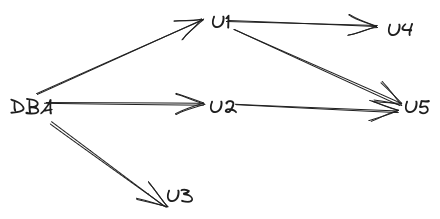
Suppose DB admin decides to revoke the authorization of $U_1$ show in Figure 14.1. Since $U_4$ has received authorization from $U_1$, his authorization should be revoked as well. However $U_5$ was granted authorization by both $U_1$ and $U_2$. Since $U_2$s authorization was not revoked $U_5$ retains the authorization.

This default behavior is cascading revokation. It can be prevented by the keyword restrict:

revoke select on department from Amit, Satoshi restrict

This revocation fails, if there are any cascading effects.

Only the privilege of granting an authorization can be revoked specifically:

revoke grant option for select on department from Amit;

Now Amit can no more grant select privilege to other users, but still has the privilege itself.

The default cascading revokation is not appropriate in many cases. Suppose Sutoshi has the role dean, grants instructor to Amit, and later dean is revoked from Sutoshi, perhaps because he leaves the University. Since Amit continues to be employed he should retain the instructor role.

To deal with this, SQL permits privilege to be granted by a role rather than by a user. SQL has a notion of the current role associated with a session. By default it is null. It can be set with

set role role_name --role associated with the session

To grant a privilege with the grantor as the current session role, we add the clause

granted by current_role

to the grant statement, provided current session role is not null.