Week 7

VL 13 - 27.05.25

Complexity (Cont.)

• we had running_mean(a, k) in O(k * N) when k = const independent from N.

• Consider two implementations, one of them uses an inappropriate data structure, and the other one a better one

  1. :

  r = [0] * len(a)
  for j in range(k - 1, len(a)):
    for i in range(j - k + 1, j + 1):
        r[j] = r[j] + get_item(a, i) # get_item(a, i) = O(i)
    r[j] /= k
  return r

  inner loop: \(\mathcal{O}(\Sigma_{i = r - j + k + 1}^{i = j + 1}(i) = \mathcal{O}(k\cdot j - k^2 / 2)) = \mathcal{O}(k\cdot j)\) (k is constant) outer loop: calculating the outer loop we get … this is the real

  2. when shifting the window there are many elements overlapping elements - recalculating the sum of each window is inefficient. Having calculated the sum of a single window, the next shift is simply obtained by removing the first element from the sum, and adding the first subsequent element outside of the window to the sum:

     r = [0] * len(a)
     for i range(k): # O(k)
        r[k - i] += a[i] 
       for j in range(k, len(a)):
        r[j] = r[j - 1] - a[j - k] + a[j]
       for j in range(k - 1, len(a)):
        r[j] /= k
       return r

  This algorithm is O(N). Slight improvement reducerd the complexity.

  Which data structure is here inappropriate? \(\Rightarrow\) linked list

Data Structures

Linked List Data Structure

a linked or doubliy linked list consists of:

class Node:
    value # data element
    next # reference to another node object

• 

  linked-list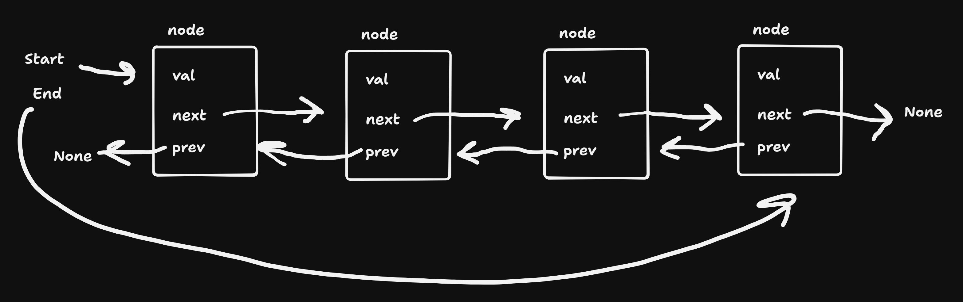

• 

  doubly linked list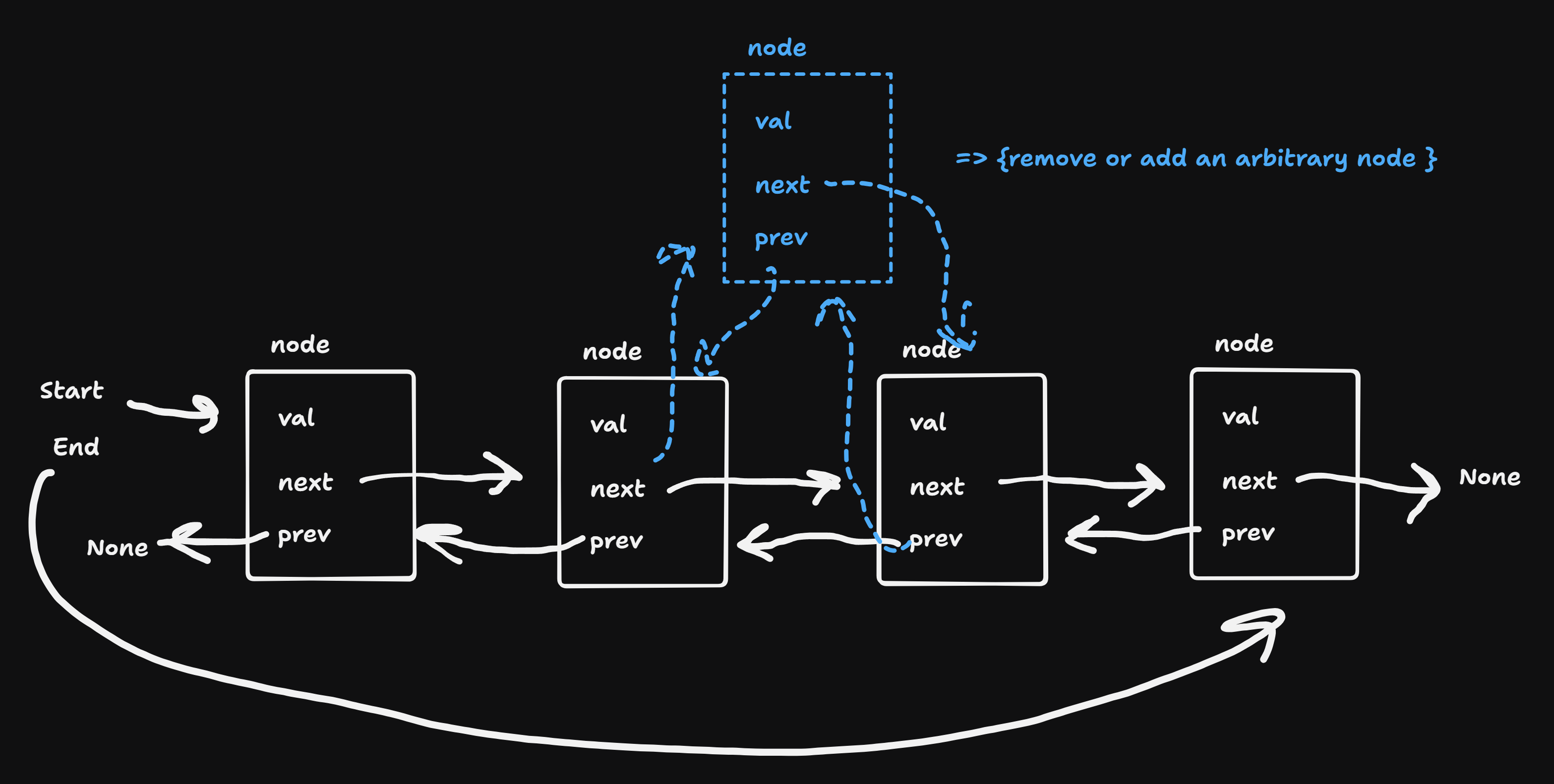

• 

  adding an element

removing an element from or adding to a linked list at an arbitrary known position is \(\mathbb{O}(1)\)

def push_front(l, v):
    n = Node()
    n.value = v
    n.next = l.start
    l.start = n

• linked list is good for inserting or removing an element at an arbitrary location
• Observation:
  • in practice it is very often sufficient to simply add elements to the end or remove from the end, reducing the importance of linked list (after the element is added at the end of the array the array can be sorted if the order is important, instead of inserting at an arbitrary location)
  • adding an element to the end of an array can be done efficiently in amortized time using dynamic arrays

Dynamic Arrays

• When appending an element to a full array, a new array with larger capacity is allocated an previous contents are copied over to the new array \(\Rightarrow\) key point. The new capacity must be a multiple of old capacity. (if it is some constant the amortzied time won’t work)
• copying is \(\mathcal{O}(N)\) but when capacity is doubled or increased depending on \(N\), this happens rarely. More precisely if the array is full, the first insert costs N. The subsequent N insert each cost 1. Thus in total N + 1 inserts cost 2N time, averaging 2 per insert. (amortized).
  • sometimes cheap: \(\mathcal{O}(1)\)
  • sometimes expensive: \(\mathcal{O}(N)\)
  \(\Rightarrow\) amortized complexity. “amortized” comes from industry or econonmics. When an expensive machine is first purchased, or a large inverstment is initially made, there is first a loss. But over time the profit of the products of the machine or the investments covers (amortizes) the initial loss.
• formally calculation with the “accounting mehtod”:
  • dynamic array data structure carries around the infomration:
    • size: amount of elements in the array
    • capacity: the total number of elements that can be stored in the array
  • let at a given time \(i\) these values be size_i and capacity_i
  • invariant of the data structure: capacity_i >= size_i
  • Define phi_i := size_i - capacity_i
  • Then the costs of an append is: c_i = c~i + (phi_i - phi(i+1))

    • case 1: there is free storage \(\Rightarrow\) size_(i - 1) < capacity_(i - 1), capacity_i = capacity_(i - 1), size_i = size_(i - 1) + 1.
      c_i = 1 + (size_i - capacity_i) - (size_(i - 1) - capacity_(i - 1)) = 1 + 1 + 2

    • case 2: capacity is full \(\Rightarrow\) double the capacity, and copy over the elements. size_i-1 = capacity_i-1, size_i = size_i-1 + 1.
      c_i~ = 1 + size_i-1, copying the elements and appending the new element

      c_i = 1 + size_i-1 + (size_i - capacity_i) - (size_i-1 - capacity_i - 1) = 1 + 1 + size_i-1 - capacity_i-1

      simplifying we obtain