Week 12

Published

July 1, 2025

VL 22 - 01.07.25

How to Represent Graphs

Nodes: whole numbers 0, …, N - 1 (or keys related to the application, e.g. Names)
Edges: Two options
1. Adjacency matrix:
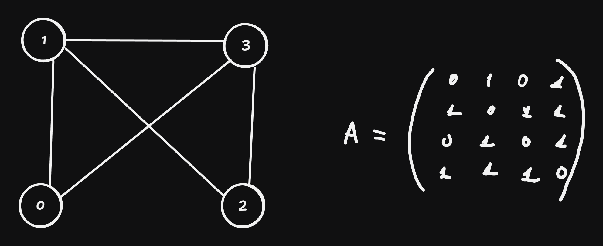
  \(A \in \{0, 1\}^{|V| \times |V|}\), s.t. \(a_{i, j} = 1 \Leftrightarrow \text{edge} i \rightarrow j \text{exixts}\)
  
  for an undirected graph: \(A = A^T\) (matri has to be symmetric)
  
  example:
  
  adjecency matrix
  
  advantages:
  - concepts and techniques can be directly applied
  - storage efficient for direct graphs that are not sparse, i.e. \(|E| \in \mathcal{O}(|V|^2)\), (but not for sparse graphs \(|E| \in \mathcal{O(|V|)}\))
2. Adjacency list: Array of arrays, an array for each node, where the arrays containes the neighbors
  
  above graph can be represented as:
  
  graph = [[1, 3], [0, 2, 3], [1, 3], [0, 1, 2]]
  - advantage: storage efficient for sparse matrices, e.g. navigation graphs
  an elegant pythonic code for a looping over all neighbours of all nodes:
```
for node, neighbors in enumerate(graph): # looping over all nodes
 for neighbor in neighbors:
    ... # do something interesting
```

Calculating the Transpose of a Graph

This means reversing all nodes.

for undirected graphs: \(G^T = G \Rightarrow A^T = A, \text{graph}^T = \text{graph}\) (graph is the adjacency list representation)

for directed graphs: \(A_{G^T} = A_G^T\) (for adjacency matrix, tranpose it.) Below we give how to tranpose the adjacency list representation of a graph:

def tranpose_graph(graph): 
 gt = [[] for i in graph]
 for node, neighbors in enumerate(graph) :
    for neighbor in neighbors :
       gt[neighbor].append(node) # reverse edges
 return gt

Traversing Graphs

Visiting all nodes (or a subset of all nodes) in a specific order.

Basics:
- Depth First Search (DFS): first traverse the depth, and then move to other neighbors
- Breadth First Search (BFS): First visit all neighbors and then go to the deeper level
Advanced:
- shortest path (dijkstra shortest path, A*-Alg): visit nodes in an increasing weight order

DFS

implementation:

def dfs(graph, start_node):
   visited = [False] * len(graph)
   def visit(node):
      if visited[node] return # node is already visited, do nothing
      visited[node] = True # register the visit
      print("discovered", node)
      for neighbor in graph[node]:
         visit[neighbor]
      print("finished", node)
   visit[start_node]

Example:

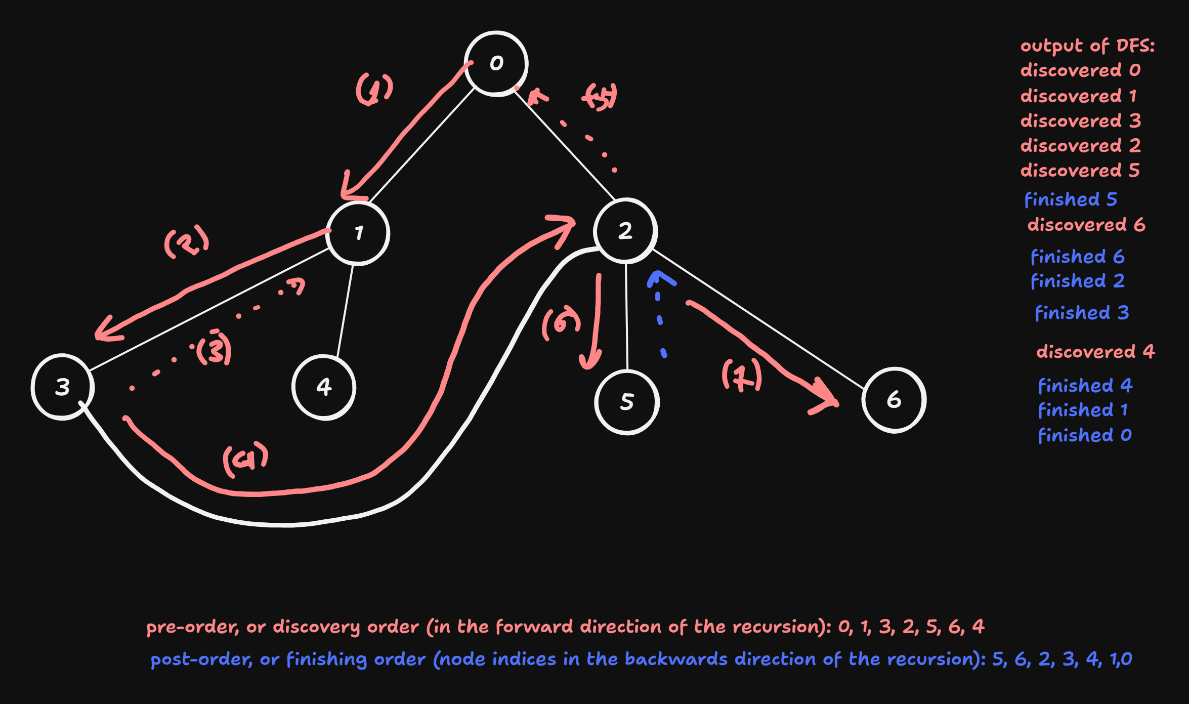
recursive implementation is elegant, but for large graphs stack depth (overflow) can be reached very easily, e.g. for graphs with thousands of nodes. But it is possible to re-write any recursive algorithm iteratively using stack data structure, and this is what we can do for DFS - we can implement it using stack data structure:

stack implementation:

from collections import deque # simultaneously a stack and a queue
def dfs(graph, start_node):
   d = deque()
   d.append(start_node)
   visited = [False] * len(graph)
   while len(d) != 0 : # there are still elements in the stack
      node = d.popright() # LIFO (for BFS we will simply replace with popleft)
      if visited[node]: continue
      visited[node] = True
      print("discovered", node)
      for neighbor in graph[node]:
         d.append(neighbor)

print("finished", node) is now not in post-order. As indicated in the comment above, to get BFS instead of DFS the only necessary difference is to change node = d.popright() to node = d.popleft().

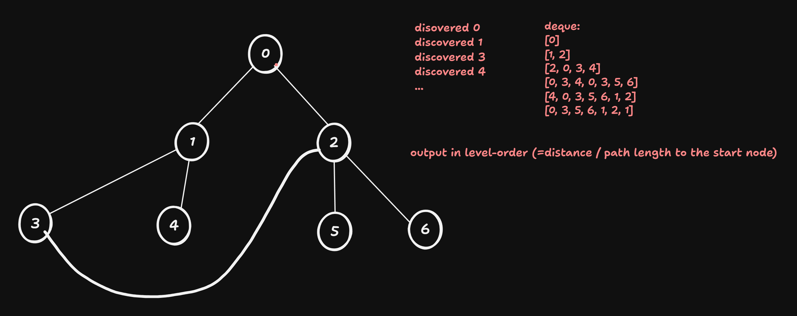
BFS

In BFS first all the neighbors are visited, and then the deeper levels. It means

replacing stack witha queue (or if a deque is used, replace popright() with popleft()).

VL 23 - 03.07.25

Applications of DFS and BFS

Copying a graph: Depth search with pre-order traversal, copying a node as soon as a node is discovered
Deleting a graph: DFS with post-order traversal

detecting whether a graph is a tree. Graph is a tree \(\Leftrightarrow\) there are no cycles

There is a cycle \(\Rightarrow\) there exists a node that can be reached in multiple ways.
A node is reached second time \(\Rightarrow\) visited[node] Flag is already True
Trivial cycles are not considered as cycles: n -> m -> n is not a cycle

implementation:

return True, is there is a cycle

def undirected_cycle_test(graph): # graph given as adjecency list
  visited = [False] * len(graph)
  def visit(node, parent):
     if not visited[node]: # no cycle
        visited[node] = True
        for neighbor in gaph[node]:
           if neighbor == parent: continue # skip trivial cycles
           if visit(neighbor, node): 
              return True
        return False
     else: return True
  return visit(0, None)

8 Queens Problem

Simplification: 4x4 chessboard with 4 queens.

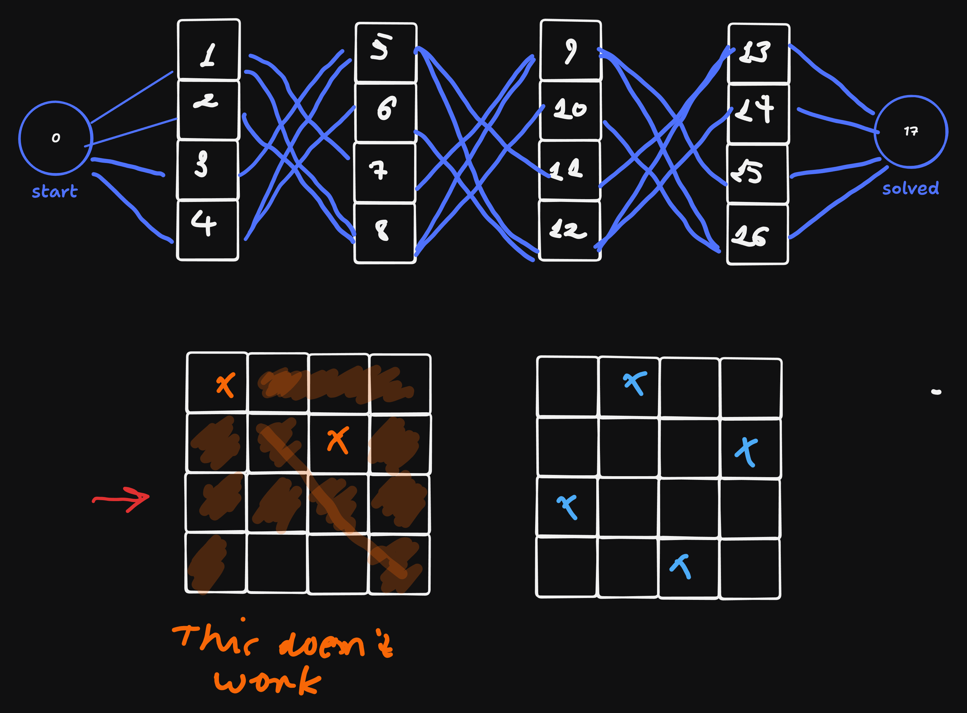
Each square is a node.

Above graph is represented as:

graph = [[1, 2, 3, 4],
         [7, 8],
         [8], ...]

Assume that we have a function check_capture(queens) solved queens: list of nodes, where the

Solution using depth search:

def place_queens(graph): 
   queens = []
   def visit(node, queens):
      if node == 17: return True # solution found
      queens.append(node) # 
      if check_capture(queens[1:]): # 
         def queens[-1]
         return False
      for neighbor in graph[node]:
         if visit[neighbor, queens]: return True
      del queens[-1]
      return False
      if visit(0, queens): return queens[1:]
      else: return None

only a single solution is found with this implementation.

All solutions

def place_quuens(graph):
   solutions = []
   queens = []
   def visit(node, queens):
      if node == 17:
         solutions.append(queens[-1])
         return
      queens.append(node)
      if not check_capture(queens[1:]): # valid partial solution
         for neightobr in graph[node]:
            visit(neighbor, queens)
      del queens[-1] # backtracking towards the next solution
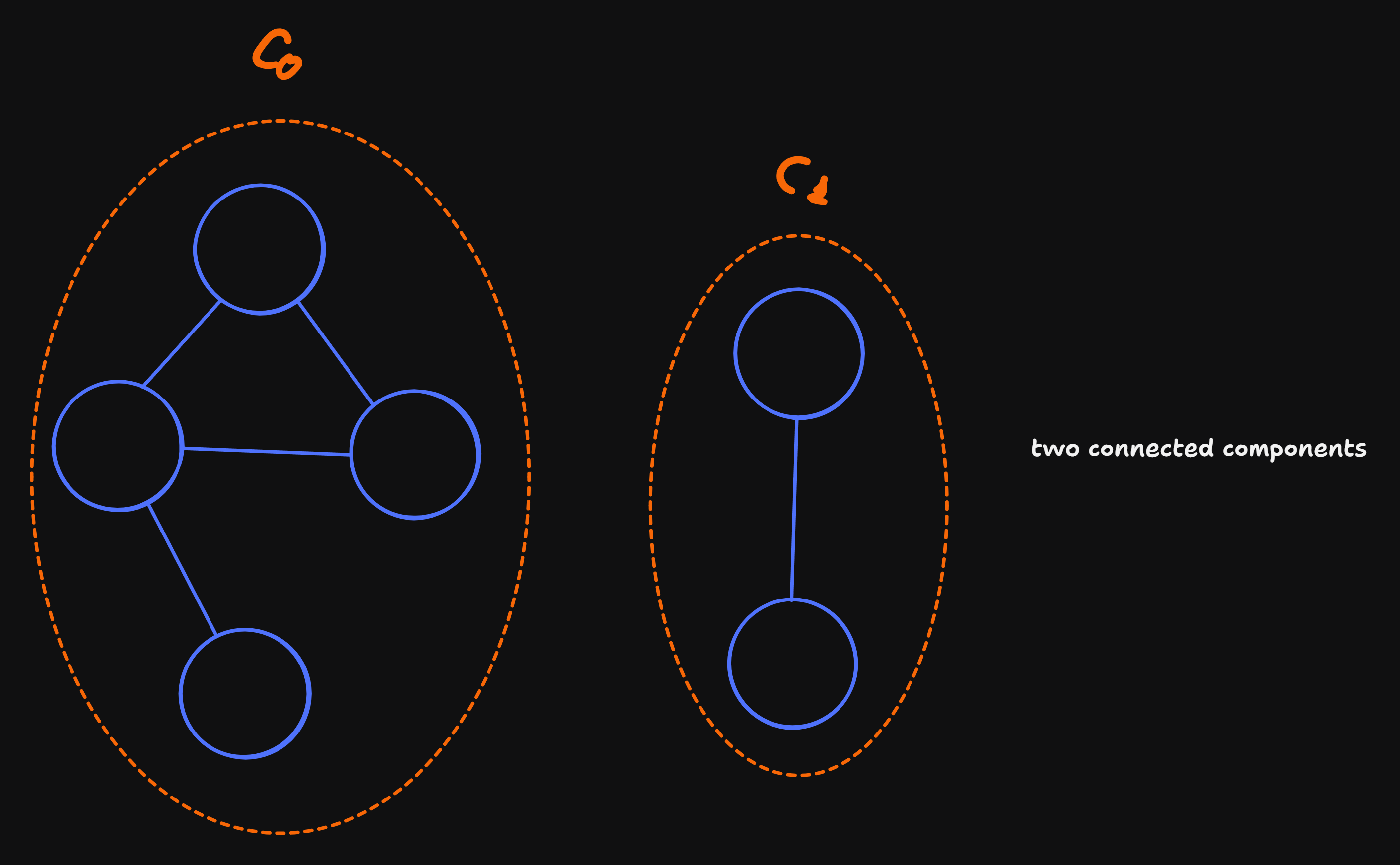
   visit(0, queens)

Searching and Identifying Connected Components

a graph is connected, if \(\forall u, v \in V\) there is a path \(u \rightsquigarrow v\)
if the graph is not connected: \(C \subset G\) is a connected component, if \(C\) is connected and \(\forall u \in V \\ C \neg u \rightsquigarrow C\)