Week 8

VL 15 - 03.06.25

Complexity (cont.)

• wenn \(f(n) in \mathcal{O}(g(N))\) dann gilt fuer die meisten ’interessanten” der Verschiebungsregel \(f(N + k) \in \mathcal{O}(g(N))\) genau dann, wenn \(f(N + k) \leq b^k \cdot f(N)\) fuer konstante \(b\) und \(N \geq N_k\) gilt.

  proof:

• Examples:

  • \(f(N) = N^D\) for \(D > 0\) (i.e. Monome, roots, …) \(f(N + k) = (N + k)^D \leq (2N)^D = 2^D\cdot N^D = 2^D\cdot f(N)\), (here we set \(N \geq k\))
  • \(f(N) = \log_a N\) \(\Rightarrow\) \(f(N + k) = \log_a (N + k) = \log_a N \cdot (1 + \frac{k}{N}) \leq ...\)
  • \(f(N) = a^N \Rightarrow f(N + k) - a^{N + k} = a^k \cdot a^N \rightarrow b = a\)

• Basically for these functions the shifting N -> N + k doesn’t change the complexity class, (algorihtm will still run longer though)

Complexity of Recursive Algorithms

Runtime: \(T(N) = T_{\text{local}}(N) + \sum_{i} T_{\text{recursive}}(N_i)\)

Two solution methods:

1. recursively substitute the definition of the formula within the sub formulas, until a simpler expression is reached. Even though this might be mathematically not exact it usually allows to guess a formula.

2. master theorem:

   master theorem can be applied when:

   \[T(N) = T_{\text{local}}(N) + a \cdot T_{\text{recursive}}(N / b)\]

   i.e. \(a\) recursive calls with smaller inputs: \(\frac{N}{b}\)

   • recursions exponent: \(\rho = \log_b a\)

     three cases:

     1. \(T_{\text{local}}(N) \in \mathcal{O}(N^{\rho - \epsilon}\), for \(\epsilon > 0\). Here the local computation is a little faster than \(N^{\rho}\). Then the complexity

        \[T(N) \in \Theta(N^{\rho})\]

     2. \(T_{\text{local}}(N) \in \Theta(N^{\rho})\). Local computation as fast as \(N^{\rho}\). Complexity:

        \[T(N) \in \Theta(N^{\rho} \log N)\]

     3. \(T_{\text{local}}(N) \in \Omega(N^{\rho + \epsilon})\), for \(\epsilon > 0\) and \(a\cdot T_{\text{local}}(\frac{N}{b}) \leq c \cdot T_{\text{local}}(N)\), s.t. \(c \leq 1\). then local computations dominate and we have:

        \[T(N) \in \Theta(T_{\text{local}}(N))\]

Searching

• the most important quality criteria of a large DB is a powerful search function
• fundamnetal search types:
  • key search ()
  • range search: keys are in an interval
  • similarity search: finds elements whose keys are similar to the given key \(\Rightarrow\)
    • correcting typing mistakes like google does it
    • content-based search (?)
  • Graph search: shortest path (navigation)

Key search

Sequential search

• when there is no order, the elements are not order by key

• advantages:

  • no requirements of specifications how the data should be stored
  • the keys must only support “==” and don’t have to support <=.

• disadvantages: slow, \(\mathcal{O}(N)\).

• general implementation:

  def sequential_search(a, target_key, key_function):
    for i in ragen(len(a)):
        if key_function(a[i]) == target_key:
            return i # or return a[i]
    return None # not found

  to simplify, we will omit the explicit usage of key_function. Then the elements themselves are the keys. But in practice usually a key function is necessary, since elements are objects or structures.

  The simplified version:

  def sequential_search(a, target_key):
    for i in range(len(a)):
        if a[i] == target_key: return i
    return None

  We want faster searching

Faster Searching Algorithms

• to have faster searching we need more information about the keys - they should support more than ==,
  • <= (total Order): binary search, \(\mathcal{O}(\log N)\)
  • hash-function: hashtable, \(\mathcal{O}(1)\)
  • quantize-function: bucketarray, \(\mathcal{O}(1)\) (or Bucket sort)

---

Binary Search

Data are in a sorted array. We need a < function.

a = [...] # define an unsorted array 
a.sort()
found = binary_search(a, key) 

• implementation:

  def binary_search_impl(a, key, start, end):
    size = end - start
    if size < 0 : return None # not found
    center = (start + end) // 2
    if a[center] == key: return center
    if a[center] < key: return binary_search_impl(a, key, center + 1, end)
    else : return binary_search_impl(a, key, start, center - 1)

  def binary_search(a, key):
    return binary_search_impl(a, key, 0, len(a)) # divide and conquer

  a = [2, 1, -3, 4]
  a.sort()
  binary_search(a, 1)

  1

Binary Search Iterative

• implementation:

def binary_search_it_impl(a, key, begin, end):
    size = end - begin
    center = (begin + end) // 2
    # invariant: key possibly in a[begin : end]
    while size != 0 :
        if a[center] == key: return center
        if key > a[center]: begin = center + 1
        if key < a[center]: end = center
        center = (begin + end) // 2
        size = end - begin
    # size == 0
    return None 

def binary_search_it(a, key):
    return binary_search_it_impl(a, key, 0, len(a))

print(a)
print(binary_search_it([3, 4], 4))

[-3, 1, 2, 4]
1

• complexity analsysi - we apply the master theorem: \(T(N) = T_{\text{local}}(N) + a T_{\text{recursive}}(\frac{N}{2})\). Then we have:
  • \(T_l = O(1)\)
  • \(a = 1\)
  • \(b = 2\)
  • \(\rho = \log_2 1 = 0 \Rightarrow L_ ...\)

VL 16 - 05.06.25

Sorting is O(nlog(n)), sequential searching of unsorted structures is O(n), which is faster. Binary search is O(log(n)) and hash table search is O(1). Binary search must be performed on a sorted structure. So if we were to resort every time we insert an element it would be less effective than sequential searching. Therefore we need a better way to keep the data structure sorted \(\Rightarrow\) Search trees

Search Trees

• Goal: inserting, removing, sorting all O(log(N))
• Def:
  • Graph:
    • nodes: data elements
    • edges: connections
  • path: a sequence of nodes where each node in the sequence are connected by an edge.
  • Tree:: any arbitrary pair of nodes are connected with a unique path. In such graphs there are no cycles.
  • Root: an arbitrarily selected node.

Tree Data Structure

tree ds

• Binary Tree: a node has at most three neighbors
  • parent: every node other than the root node (that was chosen arbitrarily) has a unique parent
  • child: every node other than the leave nodes have children
  • leaf: nodes that don’t have children
  • interior node:
  • sub-tree: in a binary tree the sub-trees get exponentially smaller (each time they are halved).

Implementation

class Node:
  def __init__(self, key, value):
    self.key = key
    self.value = value
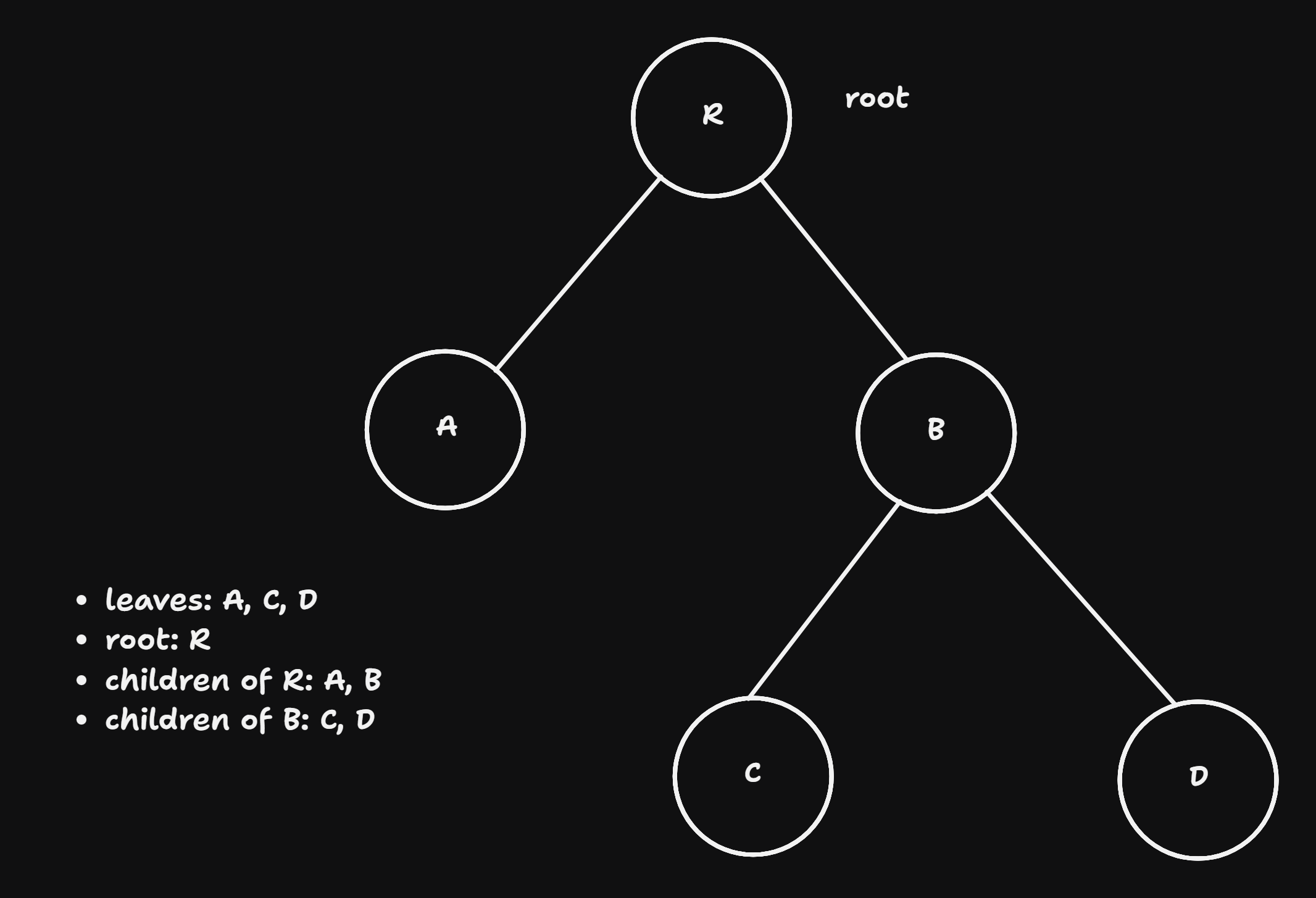
    self.left = self.right = None # a node is initially a leaf

Example construction of a tree (to simplify we omit value, i.e. keys are values themselves):

root =  Node("R")
root.left = Node("A")
root.right = Node("B")
root.right.left = Node("C")
root.right.right = Node("D")

• binary tree \(\Rightarrow\) binary search Tree when Search tree conditions are satisfied. Search tree conditions:
  1. keys are totally ordered
  2. for each node holds:
     1. all the nodes in the left substree are smaller or equal
     2. all the nodes in right substree are greater
• tree search: recursively:
  • if the target_key is greater than the ucrrent node: search in right subtree
  • otherwise search in the left subtree

implementation:

def tree_serch(node, target_key):
  if node is None: return None
  if node.key == target_key: return node
  if target_key < node.key: return tree_search(node.left, target_key)
  else return tree_search(node.right, target_key)

The tree should be maintained s.t. the search tree condition is always true and the tree is balanced. If the tree is not balanced it deteriorates to a linear search.

• Insertion: Elements should be inserted s.t. the search tree condition is always satisfied.

  • if target key larger / smaller then current key: insert in right / left subtree
  • what to do when the key is already there?
    • option1: raise error (not a good solution)
    • overwrite the data value with the new data value (this is what’s done in arrays anyways. )

• Implementation:

  def tree_insert(node, key, value):
    if node is None: return Node(key, value)
    if node.key == key:
      node.value = value # return value 
      return node
    if key < node.key:
      node.left = tree_insert(node.left, key, value)
    else:
      node.right = tree_inssert(node.right, key, value)
    return node

• bad sequnces of insertions cna cause a tree to detoriarete to a linked list:

# good sequence
root = None
root =  tree_insert(root, 4)
root = tree_insert(root, 2)
root = tree_insert(root, 3)
root = tree_insert(root, 3)
root = tree_insert(root, 6)

# bad sequence: 2, 3, 4, 6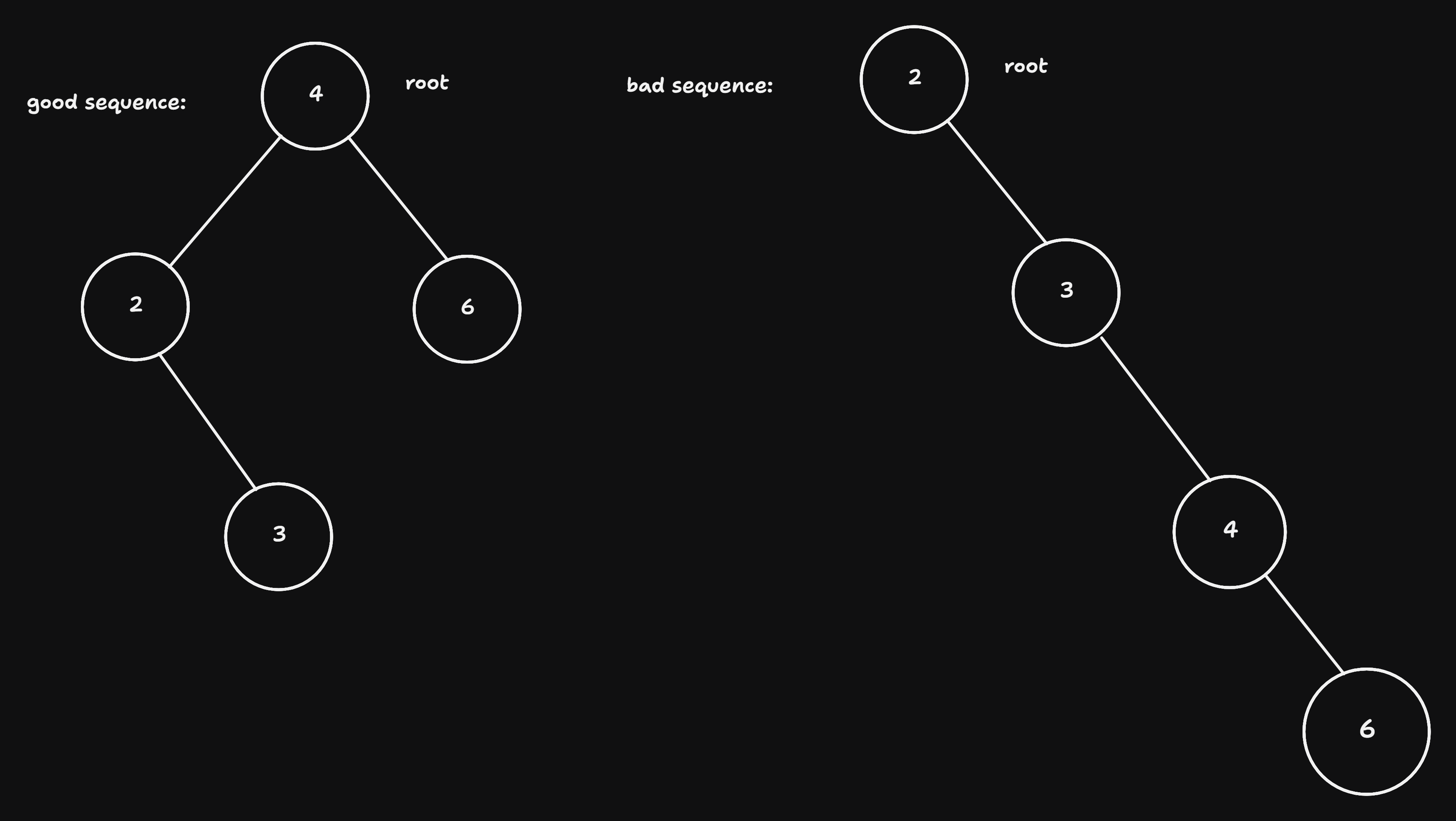

good & bad sequences

• Deletion: deletion should preserve the search condition:
  • case 0: key doesn’t exist: raise error or don’t do anything
  • case 1: key is a leaf: remove the leaf (set it to None)
  • case 2: node has a single child: replace the none
  • case 3: node has two children (difficult case)
    • search for neighbors (predeccessor or successor) of the node in the order and replace it
    • remove the neighbors of its children form the prefvious posisiont

# hilfsfunction for predecossor
def tree_predecessor(node): 
  node = node.left
  while node right is not None:
    node = node.right
  return node

def tree_remove(node, key):
  if node is None: return None # 0th case
  if key < node.key: node.left = tree_remove(node.left, key) # 
  elif key > node.key: node.right = tree_remove(node.right, key)
  else: # key == node.key
    if node.left is None and node.right is None: return None # 1st case
    if node.left is None: return node.right
    if node.right is None: return node.left
    pred = tree_predecessor(node)
    node.key = pred.key; node.value = pred.value # copy the predecessor
    node.left = tree_remove(node.left, pred.key) # remove old predecessor
    return node